following our latest discoveries, we’ll go further with lines & segments and talk about non-parallel lines.

first let me clarify one thing. if you’ve followed the previous articles, you may have noticed that I keep talking about dimensions. it is because one of the key notions of generative art is complexity.

quoting Philip Galanter in Complexity Theory as a Context for Art Theory (must read)

Generative art refers to any art practice where the artist uses a system, such as a set of natural language rules, a computer program, a machine, or other procedural invention, which is set into motion with some degree of autonomy contributing to or resulting in a completed work of art.

complexity is therefore a combination of simple elements. that’s why I used the notion of dimensions: taken separately, thickness, alpha, width, height and even time, are simple linear factors. they are easy to quantify and manipulate. once they are combined together, the result can become extremely intricate and hard to analyze. thinking of those factors as distinct dimensions helped me understand better how to get them to work together.

in the next articles we’ll study more and more complex systems, starting right now with the polyline.

with a second non parallel line we open the gate to a huge lot of variations.
as seen in the points distribution article, there are dozens of ways to distribute points.
the most basic approach is to use random set of points and create random lines by picking 2 points at random:

click to reset lines.
this is not really interesting, isn’t it ? the most important thing after choosing how to distribute points, is usually to find how to link them.

for each distribution with X being the number of points, we can draw ( ( X * ( X – 1 ) ) / 2 ) unique lines. it is known as the handshake problem and I think this solution was found by Carl Friedrich Gauss when he was a kid, there exists more than a 100 versions of this story.

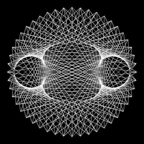
to help us figure out how complex it can become, let’s try to draw all the unique lines with 3 sets of 10, 30 and a 100 points.

10 points – 45 single connections

30 points – 435 single connections

100 points – 4950 single connections

the line count is so high that we can’t read them anymore.

doing this by hand might sound crazy yet standing in front of this 60*60 inches hand drawn piece (36 points, 630 lines) by Mark Dagley or the plexus series by Gabriel Dawe must be something.

this being said, we can use different sets of points and set some rules to have them more or less sorted. for instance using 2 circular distributions with the same amount of points (100) and different radii will give us this.

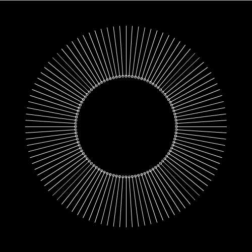
no big surprise, each origin on the inner circle corresponds to a destination on the outer circle. slightly changing the points count of the inner ( IC ) / outer ( OC ) circles will greatly impact the output say IC: 120 / OC : 30 gives

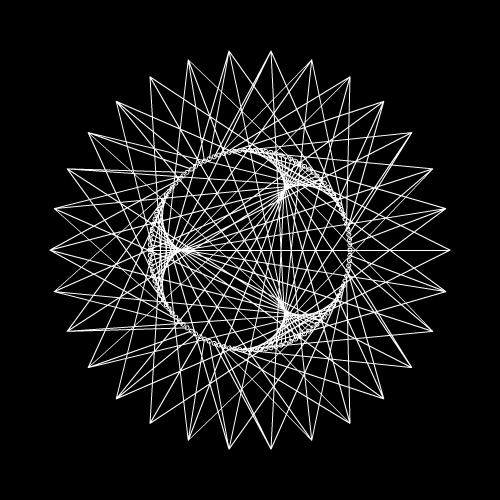
changing the X/Y radii will also greatly impact the output say IC: 240, OC : 48, RX: 200, RY : 100 gives

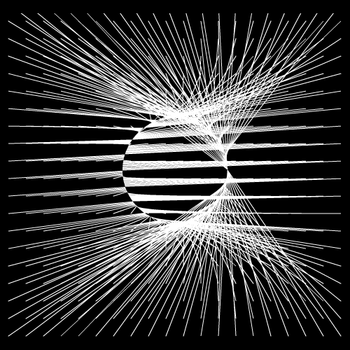
now the good thing with distributing points, is that we can use any distribution method as an input/output for instance the input is a grid distribution and the output is a circle.

this is nice already, rather graphic and easy to set up.
lines are very good at creating space or representing portions of space. they usually give a strong feeling of motion.

until now we’ve use disconnected lines, time for us to move forward and start playing with polylines. here’s a polyline:

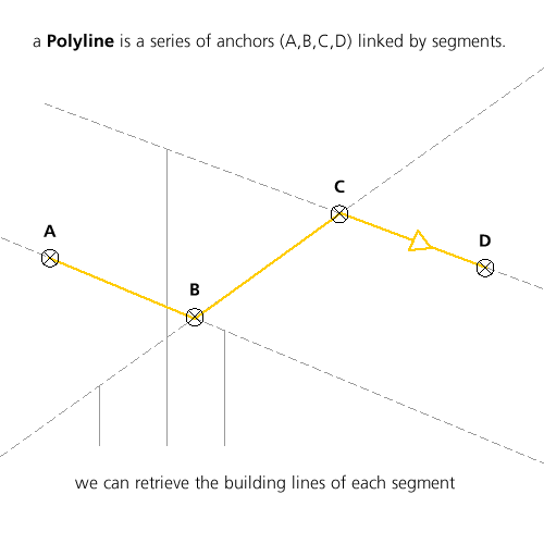
a polyline has a bunch of properties amongst which those are crucial for us:

• anchors & segments are connected
• it can be smoothed (or subdivided)
• it can be simplified
• each segment has a direction therefore a left side and a right side

polylines are used in a variety of apps ranging from games to data vizualization, graphs, maps, morphomathematics [ long list here ]. a basic overview would look like this:
give focus then left/right to navigate + up to reset

• 0 – a random set of points, we create a random polyline by picking 10 points at random
• 1 – same as above but we render it with the graphics.curveTo() method instead of the lineTo
• 2 – same as above but we use a method by Philippe Elsass the Parametric path drawing that gives nice smooth corners.
• 3 – finally, we can also draw arcs

as said above, a polyline can be smoothed, we use the anchors as handles for the spline. there are different ways to do that each of which have graphic qualities.

give the focus then drag the handles to see how the curve reacts, click somewhere to add handles. press any key to reset.

• red line is a cubic bezier, the most common method to smooth 3 or more points
• yellow line is a quadratic bezier, I think they use it in Illustrator. the segments can be thought of as control points. notice how the curve moves when folded.
• blue line is a natural cubic curve, a previous article describes it indepth. its principal quality is to run through the handles.
• green line is a Catmull Rom Spline, I’m using Makc implementation available here Catmull-Rom spline through N points

the thin line pointing at your mouse is the shortest distance to the curve, the circle indicates this position on the spline. the good thing with a smoothed polyline is that it is ALSO a polyline. the same goes for the simplification process, it was used here if you want to see what it looks like.

enough for the lines, onwards to the next step: *surprise* !

Tags: basics, generative, generative art, introduction, line