this article was initially published on Medium, I’m posting it here for the record.
PCG, data and space
1. PROCEDURAL CONTENT GENERATION (PCG)
The essence of generative design is to use functions — simple, independent actions — and algorithms — series of actions required to solve a given task — to build systems that create series of non-repeating results. PCGs encompass the programmatic generation of content, they often rely on pseudo-random data and are essentially the task of designing a process rather than an object. PCGs are massively used in object design, games, art, vfx, architecture…
DATA / SPACE / PROCESS
The coding platform, the language, the tools & tool-chain, the capture devices & data sources are irrelevant. This will obviously have an impact on the final result if chosen poorly but it is of no importance when designing a generative system. Generating things with code is language & platform agnostic.
On the other hand, there are 3 important things to take into account when generating something with code: the data you’ll be using, the space in which they’ll be displayed and the process that will transform the data.
A generative system should allow you to perform the following tasks:
modelisation: create the model of a system
simulation: use the model to process data
exploration: alter the model’s and or the simulation’s parameter
visualization: rendering the simulation as 2D or 3D graphics, video, tangible objects, installations…
DOWNSIDES
- the mathematical uniqueness is not enough to create significant differences between outcomes
- it is hard to maintain consistent variations while using numerous variables
- it is hard to assess “good” settings, human curation is often required
UPSIDES
- PCGs are very good at serial content
- the computer does the boring part
- few parameters give many variations
- emergent behaviors can produce surprising or unexpected results
Kate Compton has written an extensive post about PCG, you’ll find lots of practical advices from a seasoned professional.
EXAMPLES
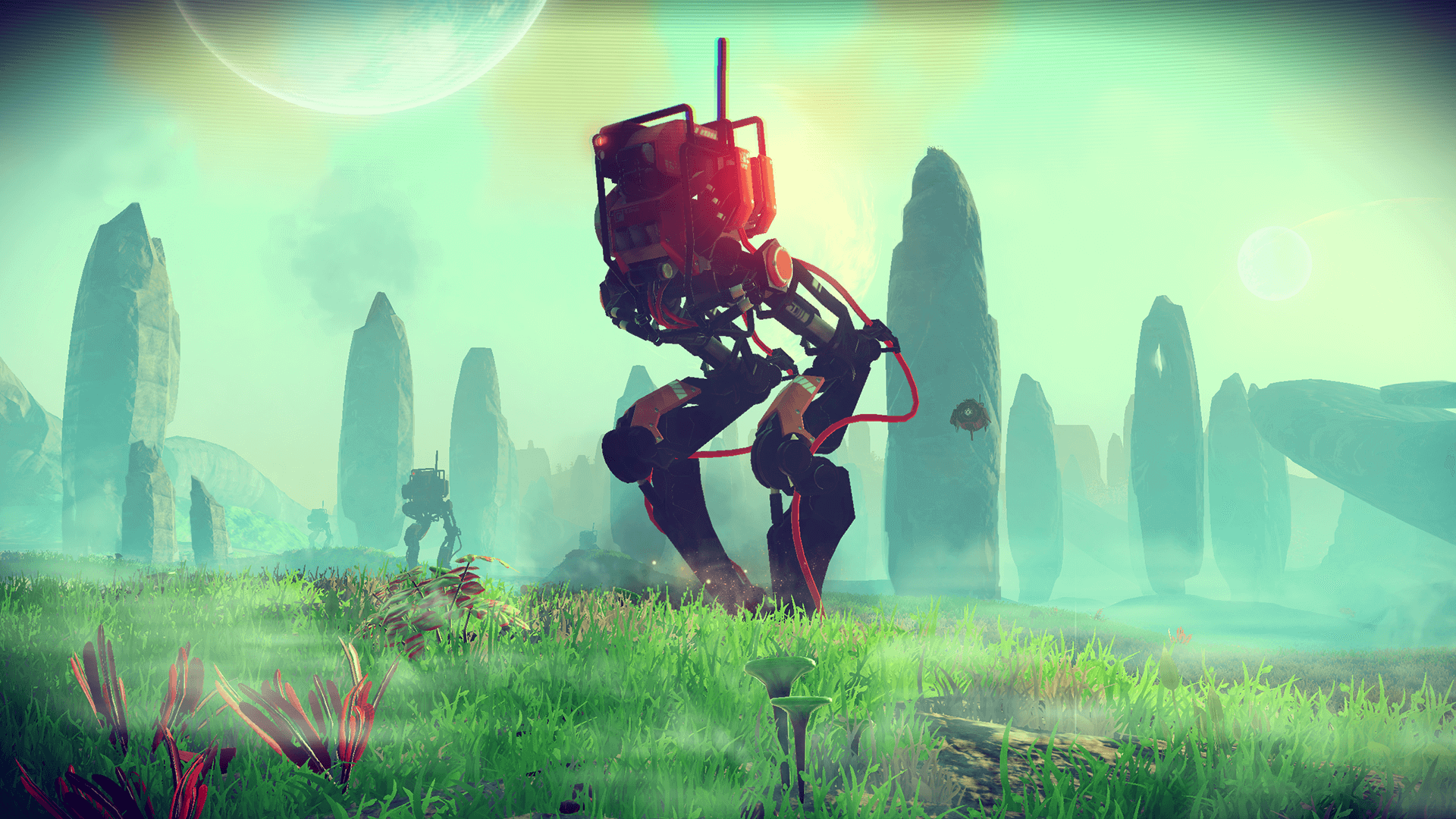
model: universe generator
simulation: update the model with game logic
exploration: interact with the simulation
visualization: rendering a 3D scene
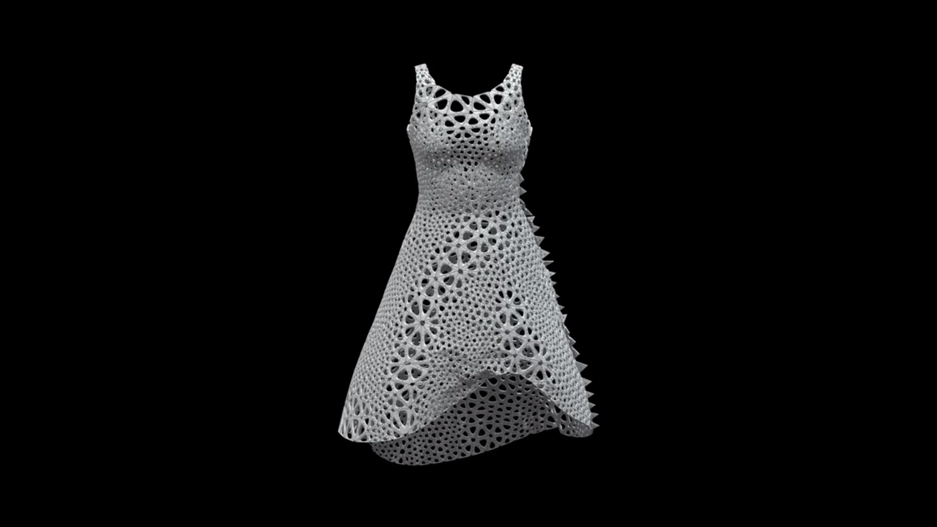
nervous systems — KINEMATICS FOLD
model: triangle based patch modeler
simulation: apply physics rules to the model
exploration: change the input 3D model
visualization: 3D renders & 3D print
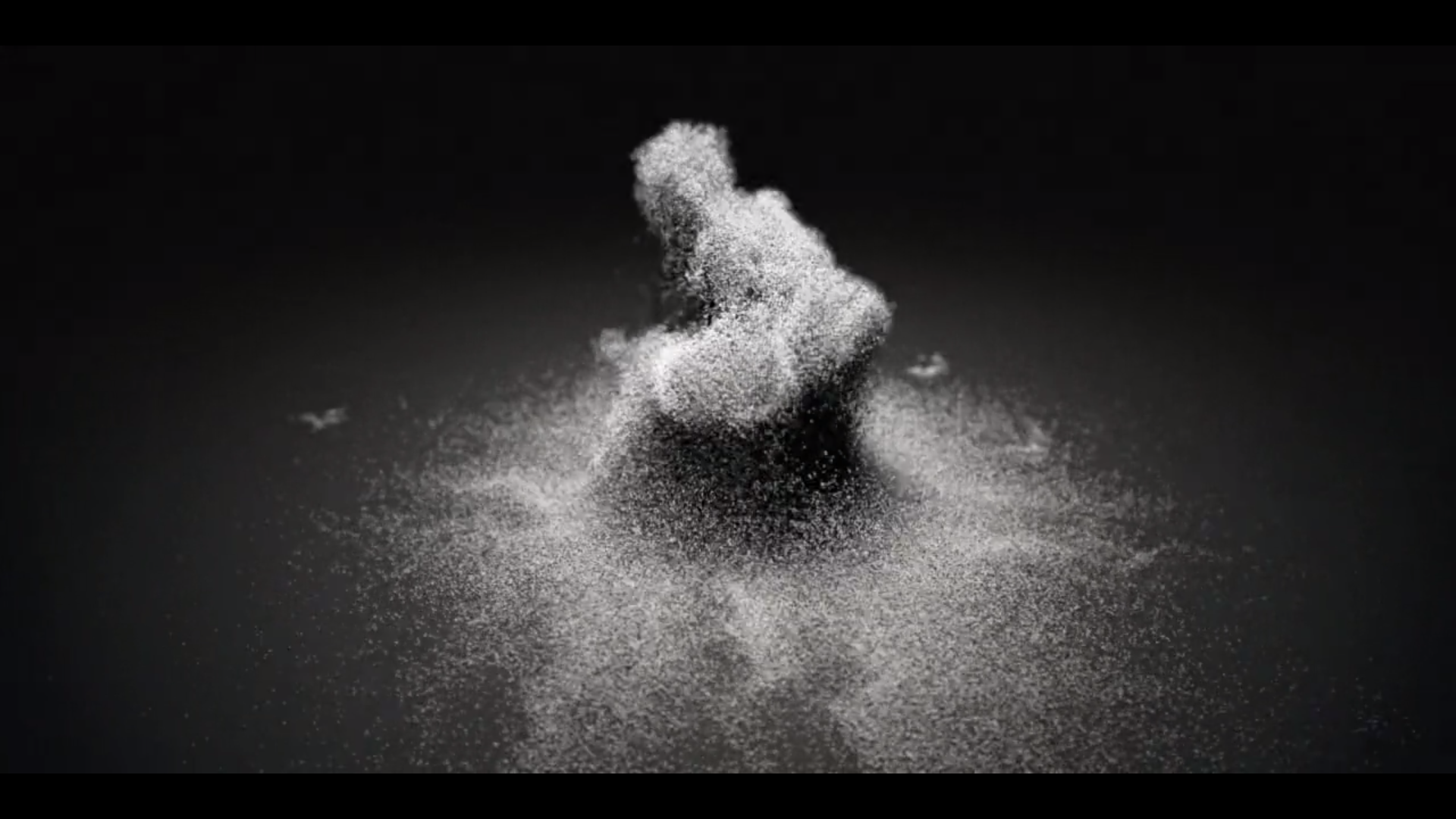
We Are Chopchop — unnamed soundsculpture
model: represent a 3D object in time and space
simulation: playback of a recorded sequence
exploration: move a virtual camera through space
visualization: render particles in 3D
In this example, the simulation’s rules — the algorithm or the system — can be described as follows:
- spawn a particle at a random location on a 3D mesh at a given time
- make the particle fall over time and chek if it hits the floor
- if the particle hits the floor, make it disappear after a while and respawn
The particles move & disappear procedurally, we know the initial position and the simulation will determine where the particle ends. This generative system can work with any 4 dimensional data set (3D position over time).
2. DATA
The universe is a continuous system yet computers need to process discretedata. In a nutshell, the difference is that continuous data are measured while discrete data are counted. The reason for that is simple ; the precision of the data that a computer works with are limited. For instance, the continuous time must become an interval for us to use it in a generative system. The light must become a color palette, a chemical reaction must be described as a process, a phenomenon will have to become a simulation etc.
Any given object can be described by a number of dimensions, in code we often refer to these dimensions as properties or fields but that’s somewhat restrictive. The values of each dimension of an object can vary without affecting the others. In the case of light, the direction, speed, wavelength and energy can vary independently ; they’re all distinct dimensions of the light and we can model and simulate them in code as the properties of an object.
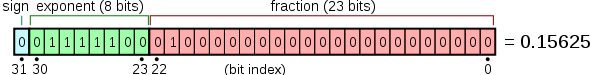
computer representation of uni-dimensional data
Once a dimension is discrete, we can use it in our models and simulations. Depending on the granularity of the dimension, we can use various data-holders the simplest of which is the bit that can only hold 2 values : 0 / 1. An obvious limitation is that it can only describe whether a given property of the object “is” or “isn’t”. If we need a finer grain, we should use different data types, what I like to call the “1D extension pack” which contains:
- byte / octet: 8 bits & 256 integer values
- float, uint, double: 16, 32, 64 bits
- character: 7 bits (US ASCII ), 32 bits (UTF-32)
acknowledged that in the computers’s memory, a number or a character is stored as an array of bits, we could argue that a number or a character are themselves N-dimensional objects.
data in 2 dimensions
The next step towards complexity is to use series of uni-dimensional data, for instance:
- a string: “Generating things with code”
- a typed linear array: [“a”, “b”, “c”] / [ 0, 1, 2 ]
- an (empty) image: [ width * height ]
the object is already multi dimensional ; each dimension can be altered without affecting the whole. The string can be longer or shorter without altering the letters, and the letters can change without altering the length of the sentence, the image’s width can change without altering its height, a.s.o.
n-dimensional data
If we extrapolate further, N-dimensional data are a combinatorics of many uni-dimensional data, here are some 3D objects:
- an opaque color: { R, G, B }
- a vector: { X, Y, Z }
- a greyscale pixel: { X, Y, greyscale }
As the name suggests, N-dimensional data can represent any number of dimensions, here are some more complex (yet fairly common) data-holders:
- pixel + color: { X, Y, R, G, B }
- pixel + color & alpha: { X, Y, R, G, B, A }
- stereo sound: { left, right, time, sampling rate }
- video: size, color depth, sound, time
- 3D object: positions, indices, normals, colors, uvs, textures…
From the dimensions’ perspective, a single tweet can potentially be represented in ~72 dimensions, often themselves N-dimensional. The underlying idea is that we often overlook the complexity of the simplest things ; a short text, a limited set of colors, an IP address are complex N-dimensional objects.
data acquisition
We are also surrounded by devices that allow us to capture rich data from our surroundings. A smartphone can capture photos, videos, sounds & GPS positions but also has a set of “hidden” sensors:
|
1 2 3 4 5 6 7 8 9 10 11 |
TYPE_ACCELEROMETER Motion detection (shake, tilt, etc.). TYPE_AMBIENT_TEMPERATURE Monitoring air temperatures. TYPE_GRAVITY Motion detection (shake, tilt, etc.). TYPE_GYROSCOPE Rotation detection (spin, turn, etc.). TYPE_LIGHT Controlling screen brightness. TYPE_LINEAR_ACCELERATION Monitoring acceleration along an axis. TYPE_MAGNETIC_FIELD Creating a compass. TYPE_ORIENTATION Determining device position. TYPE_PRESSURE Monitoring air pressure changes. TYPE_PROXIMITY Phone position during a call. TYPE_RELATIVE_HUMIDITY Monitoring absolute & relative humidity. |
All these sensors (and more) are readily accessible and can be recorded from the smartphones as an input to our generative system.
The open data available to us have grown exponentially for the past years, they are rather oriented towards statistical analysis, mostly “geo-social” and often geolocated. This is especially true for cartography but not only.
We can also use some tracking devices such as a webcam or a microphone as with a smartphone but also mainstream devices like a Kinect (video, depth, 3D point clouds, infrared video, skeletal information), the Leap Motion that precisely scans a smaller area and returns a well defined point cloud and descriptors for hands and fingers positions. More recently the VR devices like the Oculus Rift (mostly 3 DOF) and the HTC Vive (room scale 6 DOF) that allow to precisely capture the orientation and position of a headset and hand held devices in space and time.
If this is’nt enough, it’s possible to build custom devices starting with Arduino boards and Processing and adding all manners of cheap sensors: gesture detection, heat detector, 360° scanners, wind, rain, smoke sensors…
And finally, let’s not forget that we can synthesize data. The most basic form of synthetic data is obviously the random, noise, fractals and turbulence generators, but other techniques have emerged in the past years that deserve a mention. Photogrammetry is one of them, it consists in re-building a 3D model from a set of 2D pictures (see visualSFM for more information). Convolutional Neural Networks, Generative Adversarial Networks, what we usually call AI that gained a huge momentum since deepdream and partially solves one of the downsides of PCGs I mentioned above ( ‘it is hard to assess “good” settings’ )
In short, there are more and more data available and they become more and more complex. Reduced to sets of uni-dimensional variables, these data can shift between various spaces.
3. SPACES
Spaces are fields of representation, a place where the data can exist. They have specific qualities that can help you highlight the traits of the data you’re using. The important thing to acknowledge is their umber of dimensions ; N-dimensional data require N-dimensional space to be fully displayed.
2D euclidean spaces
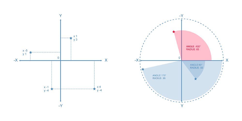
The 2D cartesian space (above left) will let you display 2D data in a simple manner based on their X and Y values. It’s the space of a page, a print or a map there is few to no work to get the data to fit and it’s easy to draw lines between data points. The polar space (above right) is a way to represent 2D data as an Angle/Radius pairs, displaying data in the 2D cartesian plane requires a simple transform ( x=sin(A)*R & y=cos(A)*R ), once transformed, you can draw lines and most graphic APIs have methods to draw arcs between data points.
3D euclidean spaces
Extending the 2D cartesian (X/Y) space to 3D is trivial, first our object needs a third dimension (Z), then we need a third dimension in space to display it. It’s the most used 3D space, it’s very intuitive to use and to understand. But there are some lesser known 3D spaces.
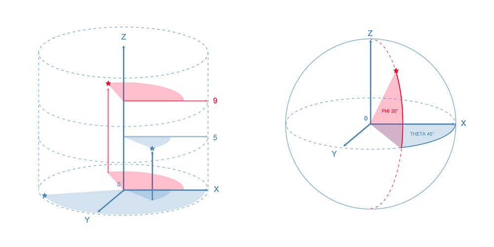
The cylindrical space (above left) and the spherical space (above right) are both extensions to the 2D polar space and a good example of what happens when you add a dimension to your data. Both data points are 3-dimensional: Angle/Radius + something. In the case of the cylindrical space, the 3rd dimension will be used to extrude the data point along the Z axis while in the spherical space, the 3rd dimension of the data point will encode a second angle that will move the data point on the Z axis as if it moved on the surface of a sphere. Two important things to note :
- data shape spaces and spaces shape data
- data can shift between spaces of same dimensions
color spaces
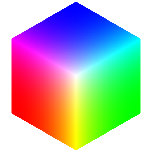
A good example of the above mentioned shift is the colors spaces. A color is usually stored as a triplet of values: Red, Green and Blue ranging from 0 to 0xFF to match the way they are used by graphic APIS (color = R<<16|G<<8|B).
As they have the same number of dimensions as a 3D point, we can map these data points directly to a 3D cartesian space where X=R, Y=G and Z=B and as we saw above, they can also be mapped to cylindrical and spherical spaces (HSL colors).
That’s a very important feature when working with generative systems ; it’s a sort of synesthesia where colors can become positions, positions can become sounds, sounds can become colors a.s.o.
higher dimensions
Colors are a good example because they have a low number of dimensions, there is at most 4: RGB + Alpha (opacity). Now what if we wanted to represent the 4th dimension of a color set? We know how to display our colors in a 3D space but what does a 4D space look like?
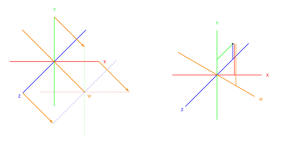
The above illustrates what a 4D space could look like, the 4th dimension (usually, the time) would be represented by the orange axis.
To represent high dimensional space data, we’ll often need to project them onto a lower dimension. This operation will obliterate the values of some dimensions, and we will have to find a way to represent the parameters that “went missing” during the projection. In the above illustration, it is very difficult to locate the points drawn on the right in the 4D space as not one but 2 dimensions went missing during the projection.
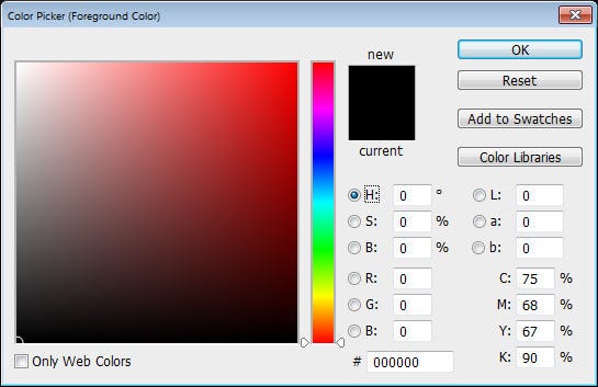
This color palette is the 2D projection of a 3D object and the spectrum ramp represents the dimension that “went missing”.
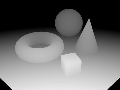
Above is the projection of a 3D scene onto a 2D surface, the depth data is lost
and a depth buffer is used to represent the “missing data” as a greyscale: the brightest the pixel, the closest our data point was to the camera. depending on the space your using, there are some strategies to reduce the dimensionality of your dataset.
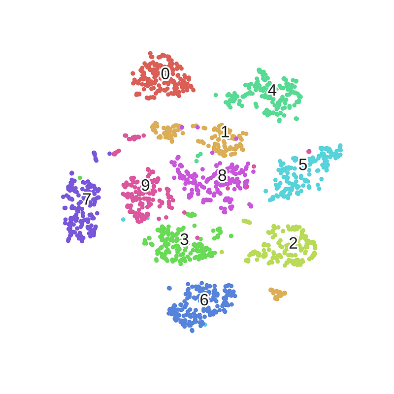
The above picture is the result of the t-SNE algorithm applied to the MNIST dataset ; high dimensional feature vectors are grouped by similarity then projected in 2D. In general, making sense of high dimensional data is hard (or lossy) and you should keep the dimensions’ count as low as possible.
other types of spaces
As a final note, there exist many other types of spaces. If we think of geometry only, the non-euclidean spaces and hyperbolic spaces are very interesting to explore (and not too hard to implement). There is of course the physical/tangible space, you’ll probably need some extra hardware like a laser cutter, a 3D printer or a CNC milling machine but holding the results of your generative system in your hands is very rewarding. Also worth noting the sound which usually requires a physical space to be explored but generates a space in space.